blackstone contains many functions for data analysis.
This vignette shows you:
How to create frequency tables for survey items and demographics with Blackstone Research and Evaluation branding.
How create composite scales from survey items with a shared underlying concept.
How to determine the if data is distributed normally.
How to run appropriate statistical tests for common data analysis tasks.
We’ll start by loading blackstone:
Read in Example Data
First, read in the data that is merged and cleaned in the vignette Importing and Cleaning Data:
# Read in clean SM data:
sm_data <- readr::read_csv(blackstone::blackstoneExample("sm_data_clean.csv"), show_col_types = FALSE)

## Set up character vectors of likert scale levels:
## Knowledge scale
levels_knowledge <- c("Not knowledgeable at all", "A little knowledgeable", "Somewhat knowledgeable", "Very knowledgeable", "Extremely knowledgeable")
## Research Items scale:
levels_confidence <- c("Not at all confident", "Slightly confident", "Somewhat confident", "Very confident", "Extremely confident")
## Ability Items scale:
levels_min_ext <- c("Minimal", "Slight", "Moderate", "Good", "Extensive")
## Ethics Items scale:
levels_agree5 <- c("Strongly disagree", "Disagree", "Neither agree nor disagree", "Agree", "Strongly agree")

# Demographic levels:
gender_levels <- c("Female","Male","Non-binary", "Do not wish to specify")
role_levels <- c("Undergraduate student", "Graduate student", "Postdoc",  "Faculty")
ethnicity_levels <- c("White (Non-Hispanic/Latino)", "Asian", "Black",  "Hispanic or Latino", "American Indian or Alaskan Native",
                      "Native Hawaiian or other Pacific Islander", "Do not wish to specify")
first_gen_levels <- c("Yes", "No", "I'm not sure")

# Use mutate() for convert each item in each scale to a factor with vectors above, across() will perform a function for items selected using contains() or can be selected
# by variables names individually using a character vector: _knowledge or use c("pre_knowledg","post_knowledge")
# Also create new numeric variables for all the likert scale items and use the suffix '_num' to denote numeric:
sm_data <- sm_data %>% dplyr::mutate(dplyr::across(tidyselect::contains("_knowledge"), ~ factor(., levels = levels_knowledge)), # match each name pattern to select to each factor level
                                     dplyr::across(tidyselect::contains("_knowledge"), as.numeric, .names = "{.col}_num"), # create new numeric items for all knowledge items
                                     dplyr::across(tidyselect::contains("research_"), ~ factor(., levels = levels_confidence)),
                                     dplyr::across(tidyselect::contains("research_"), as.numeric, .names = "{.col}_num"), # create new numeric items for all research items
                                     dplyr::across(tidyselect::contains("ability_"), ~ factor(., levels = levels_min_ext)),
                                     dplyr::across(tidyselect::contains("ability_"), as.numeric, .names = "{.col}_num"), # create new numeric items for all ability items
                                     # select ethics items but not the open_ended responses:
                                     dplyr::across(tidyselect::contains("ethics_") & !tidyselect::contains("_oe"), ~ factor(., levels = levels_agree5)),
                                     dplyr::across(tidyselect::contains("ethics_") & !tidyselect::contains("_oe"), as.numeric, .names = "{.col}_num"), # new numeric items for all ethics items
                                     # individually convert all demographics to factor variables:
                                     gender = factor(gender, levels = gender_levels),
                                     role = factor(role, levels = role_levels),
                                     ethnicity = factor(ethnicity, levels = ethnicity_levels),
                                     first_gen = factor(first_gen, levels = first_gen_levels),
                                     )
sm_data
#> # A tibble: 100 × 98
#>   respondent_id collector_id start_date end_date   ip_address      email_address
#>           <dbl>        <dbl> <date>     <date>     <chr>           <chr>
#> 1  114628000001    431822954 2024-06-11 2024-06-12 227.224.138.113 coraima59@me…
#> 2  114628000002    431822954 2024-06-08 2024-06-09 110.241.132.50  mstamm@hermi…
#> 3  114628000003    431822954 2024-06-21 2024-06-22 165.58.112.64   precious.fei…
#> 4  114628000004    431822954 2024-06-08 2024-06-09 49.34.121.147   ines52@gmail…
#> 5  114628000005    431822954 2024-06-02 2024-06-03 115.233.66.80   franz44@hotm…
#> # ℹ 95 more rows
#> # ℹ 92 more variables: first_name <chr>, last_name <chr>, unique_id <dbl>,
#> #   pre_knowledge <fct>, pre_research_1 <fct>, pre_research_2 <fct>,
#> #   pre_research_3 <fct>, pre_research_4 <fct>, pre_research_5 <fct>,
#> #   pre_research_6 <fct>, pre_research_7 <fct>, pre_research_8 <fct>,
#> #   pre_ability_1 <fct>, pre_ability_2 <fct>, pre_ability_3 <fct>,
#> #   pre_ability_4 <fct>, pre_ability_5 <fct>, pre_ability_6 <fct>, …
Likert Scale Table
The most common task is creating frequency tables of counts and
percentages for likert scale items, blackstone has the
likertTable() for that:
# Research items pre and post frequency table, with counts and percentages: use levels_confidence character vector
# use likertTable to return frequency table, passing the scale_labels: (can also label the individual questions using the arg question_label)
sm_data %>% dplyr::select(tidyselect::contains("research_") & !tidyselect::contains("_num") & where(is.factor)) %>%
                blackstone::likertTable(., scale_labels = levels_confidence)
Question |
Not at all |
Slightly |
Somewhat |
Very |
Extremely |
n |
|---|---|---|---|---|---|---|
pre_research_1 |
10 (10%) |
8 (8%) |
41 (41%) |
27 (27%) |
14 (14%) |
100 |
pre_research_2 |
56 (56%) |
19 (19%) |
8 (8%) |
9 (9%) |
8 (8%) |
100 |
pre_research_3 |
32 (32%) |
23 (23%) |
15 (15%) |
20 (20%) |
10 (10%) |
100 |
pre_research_4 |
9 (9%) |
24 (24%) |
32 (32%) |
24 (24%) |
11 (11%) |
100 |
pre_research_5 |
40 (40%) |
18 (18%) |
21 (21%) |
13 (13%) |
8 (8%) |
100 |
pre_research_6 |
17 (17%) |
25 (25%) |
25 (25%) |
16 (16%) |
17 (17%) |
100 |
pre_research_7 |
59 (59%) |
13 (13%) |
11 (11%) |
10 (10%) |
7 (7%) |
100 |
pre_research_8 |
21 (21%) |
19 (19%) |
23 (23%) |
19 (19%) |
18 (18%) |
100 |
post_research_1 |
2 (2%) |
26 (26%) |
23 (23%) |
25 (25%) |
24 (24%) |
100 |
post_research_2 |
12 (12%) |
14 (14%) |
12 (12%) |
14 (14%) |
48 (48%) |
100 |
post_research_3 |
8 (8%) |
22 (22%) |
21 (21%) |
23 (23%) |
26 (26%) |
100 |
post_research_4 |
2 (2%) |
24 (24%) |
25 (25%) |
19 (19%) |
30 (30%) |
100 |
post_research_5 |
14 (14%) |
19 (19%) |
19 (19%) |
19 (19%) |
29 (29%) |
100 |
post_research_6 |
5 (5%) |
3 (3%) |
24 (24%) |
28 (28%) |
40 (40%) |
100 |
post_research_7 |
11 (11%) |
10 (10%) |
14 (14%) |
17 (17%) |
48 (48%) |
100 |
post_research_8 |
4 (4%) |
7 (7%) |
23 (23%) |
23 (23%) |
43 (43%) |
100 |
Using Functional Programming to Speed Up Analysis
Here is one approach to use functional programming from the purrr package create many frequency tables at once:
# Another way to make a list of many freq_tables to print out with other data analysis later on,
# using pmap() to do multiple likertTable() at once:
# Set up tibbles of each set of scales that contain all pre and post data:
# research:
research_df <- sm_data %>% dplyr::select(tidyselect::contains("research_") & !tidyselect::contains("_num") & where(is.factor))
# knowledge:
knowledge_df <- sm_data %>% dplyr::select(tidyselect::contains("_knowledge") & !tidyselect::contains("_num") & where(is.factor))
# ability:
ability_df <- sm_data %>% dplyr::select(tidyselect::contains("ability_") & !tidyselect::contains("_num") & where(is.factor))
# ethics:
ethics_df <- sm_data %>% dplyr::select(tidyselect::contains("ethics_") & !tidyselect::contains("_oe") & !tidyselect::contains("_num") & where(is.factor))

# set up tibble with the columns as the args to pass to likertTable(), each row of the column `df` is the tibble of items and
# each row of `scale_labels` is the vector of likert scale labels:
freq_params <- tibble::tribble(
  ~df,           ~scale_labels, # name of columns (these need to match the names of the arguments in the function that you want to use later in `purrr::pmap()`)
   knowledge_df,  levels_knowledge,
   research_df,   levels_confidence,
   ability_df,    levels_min_ext,
   ethics_df,     levels_agree5
)
# Create a named list of frequency tables by using `purrr::pmap()` which takes in a tibble where each column is an argument that is passed to the function, and
# each row is contains the inputs for a single output, so here each row will be one frequency table that is return to a list and named for easy retrieval later on:
freq_tables <- freq_params %>% purrr::pmap(blackstone::likertTable) %>%
    purrr::set_names(., c("Knowledge Items", "Research Items", "Ability Items", "Ethics Items"))

# Can select the list by position or by name:
# freq_tables[[1]] # by list position
freq_tables[["Knowledge Items"]] # by name
Question |
Not |
A little |
Somewhat |
Very |
Extremely |
n |
|---|---|---|---|---|---|---|
pre_knowledge |
65 (65%) |
11 (11%) |
9 (9%) |
9 (9%) |
6 (6%) |
100 |
post_knowledge |
7 (7%) |
14 (14%) |
9 (9%) |
24 (24%) |
46 (46%) |
100 |
freq_tables[["Research Items"]]Question |
Not at all |
Slightly |
Somewhat |
Very |
Extremely |
n |
|---|---|---|---|---|---|---|
pre_research_1 |
10 (10%) |
8 (8%) |
41 (41%) |
27 (27%) |
14 (14%) |
100 |
pre_research_2 |
56 (56%) |
19 (19%) |
8 (8%) |
9 (9%) |
8 (8%) |
100 |
pre_research_3 |
32 (32%) |
23 (23%) |
15 (15%) |
20 (20%) |
10 (10%) |
100 |
pre_research_4 |
9 (9%) |
24 (24%) |
32 (32%) |
24 (24%) |
11 (11%) |
100 |
pre_research_5 |
40 (40%) |
18 (18%) |
21 (21%) |
13 (13%) |
8 (8%) |
100 |
pre_research_6 |
17 (17%) |
25 (25%) |
25 (25%) |
16 (16%) |
17 (17%) |
100 |
pre_research_7 |
59 (59%) |
13 (13%) |
11 (11%) |
10 (10%) |
7 (7%) |
100 |
pre_research_8 |
21 (21%) |
19 (19%) |
23 (23%) |
19 (19%) |
18 (18%) |
100 |
post_research_1 |
2 (2%) |
26 (26%) |
23 (23%) |
25 (25%) |
24 (24%) |
100 |
post_research_2 |
12 (12%) |
14 (14%) |
12 (12%) |
14 (14%) |
48 (48%) |
100 |
post_research_3 |
8 (8%) |
22 (22%) |
21 (21%) |
23 (23%) |
26 (26%) |
100 |
post_research_4 |
2 (2%) |
24 (24%) |
25 (25%) |
19 (19%) |
30 (30%) |
100 |
post_research_5 |
14 (14%) |
19 (19%) |
19 (19%) |
19 (19%) |
29 (29%) |
100 |
post_research_6 |
5 (5%) |
3 (3%) |
24 (24%) |
28 (28%) |
40 (40%) |
100 |
post_research_7 |
11 (11%) |
10 (10%) |
14 (14%) |
17 (17%) |
48 (48%) |
100 |
post_research_8 |
4 (4%) |
7 (7%) |
23 (23%) |
23 (23%) |
43 (43%) |
100 |
freq_tables[["Ability Items"]]Question |
Minimal |
Slight |
Moderate |
Good |
Extensive |
n |
|---|---|---|---|---|---|---|
pre_ability_1 |
9 (9%) |
28 (28%) |
37 (37%) |
15 (15%) |
11 (11%) |
100 |
pre_ability_2 |
24 (24%) |
14 (14%) |
27 (27%) |
22 (22%) |
13 (13%) |
100 |
pre_ability_3 |
26 (26%) |
30 (30%) |
19 (19%) |
19 (19%) |
6 (6%) |
100 |
pre_ability_4 |
43 (43%) |
27 (27%) |
13 (13%) |
4 (4%) |
13 (13%) |
100 |
pre_ability_5 |
32 (32%) |
18 (18%) |
26 (26%) |
17 (17%) |
7 (7%) |
100 |
pre_ability_6 |
26 (26%) |
12 (12%) |
18 (18%) |
26 (26%) |
18 (18%) |
100 |
post_ability_1 |
3 (3%) |
20 (20%) |
23 (23%) |
20 (20%) |
34 (34%) |
100 |
post_ability_2 |
2 (2%) |
11 (11%) |
11 (11%) |
29 (29%) |
47 (47%) |
100 |
post_ability_3 |
11 (11%) |
19 (19%) |
22 (22%) |
15 (15%) |
33 (33%) |
100 |
post_ability_4 |
9 (9%) |
6 (6%) |
9 (9%) |
23 (23%) |
53 (53%) |
100 |
post_ability_5 |
12 (12%) |
19 (19%) |
16 (16%) |
27 (27%) |
26 (26%) |
100 |
post_ability_6 |
6 (6%) |
11 (11%) |
29 (29%) |
29 (29%) |
25 (25%) |
100 |
freq_tables[["Ethics Items"]]Question |
Strongly |
Disagree |
Neither |
Agree |
Strongly |
n |
|---|---|---|---|---|---|---|
pre_ethics_1 |
10 (10%) |
16 (16%) |
45 (45%) |
20 (20%) |
9 (9%) |
100 |
pre_ethics_2 |
20 (20%) |
15 (15%) |
27 (27%) |
23 (23%) |
15 (15%) |
100 |
pre_ethics_3 |
28 (28%) |
16 (16%) |
30 (30%) |
12 (12%) |
14 (14%) |
100 |
pre_ethics_4 |
50 (50%) |
17 (17%) |
12 (12%) |
6 (6%) |
15 (15%) |
100 |
pre_ethics_5 |
14 (14%) |
16 (16%) |
31 (31%) |
30 (30%) |
9 (9%) |
100 |
post_ethics_1 |
4 (4%) |
18 (18%) |
24 (24%) |
30 (30%) |
24 (24%) |
100 |
post_ethics_2 |
7 (7%) |
10 (10%) |
13 (13%) |
31 (31%) |
39 (39%) |
100 |
post_ethics_3 |
7 (7%) |
26 (26%) |
14 (14%) |
28 (28%) |
25 (25%) |
100 |
post_ethics_4 |
10 (10%) |
7 (7%) |
6 (6%) |
19 (19%) |
58 (58%) |
100 |
post_ethics_5 |
3 (3%) |
14 (14%) |
25 (25%) |
31 (31%) |
27 (27%) |
100 |
Grouped Demograpic Table
blackstone contains a function to create frequency
tables for demographics (combined demographics table) that can also be
grouped by a variable, like role or cohort as well:
groupedTable().
# Set up labels for variables
# Labels for questions column of table, pass to question_labels argument:
demos_labels <- c('Gender' = "gender",
                  "Role" = "role",
                  'Race/Ethnicity' = "ethnicity",
                  'First-Generation College Student' = "first_gen")

sm_data %>% dplyr::select(gender, role, ethnicity, first_gen) %>% # select the demographic vars
                 blackstone::groupedTable(question_labels = demos_labels) # pass the new labels for the 'Question' column.
Question |
Response |
n = 1001 |
|---|---|---|
Gender |
||
Female |
53 (53%) |
|
Male |
46 (46%) |
|
Non-binary |
1 (1%) |
|
Role |
||
Undergraduate student |
48 (48%) |
|
Graduate student |
23 (23%) |
|
Postdoc |
21 (21%) |
|
Faculty |
8 (8%) |
|
Race/Ethnicity |
||
White (Non-Hispanic/Latino) |
43 (43%) |
|
Asian |
11 (11%) |
|
Black |
18 (18%) |
|
Hispanic or Latino |
12 (12%) |
|
American Indian or Alaskan Native |
7 (7%) |
|
Native Hawaiian or other Pacific Islander |
7 (7%) |
|
Do not wish to specify |
2 (2%) |
|
First-Generation |
||
Yes |
51 (51%) |
|
No |
47 (47%) |
|
I'm not sure |
2 (2%) |
|
1n (%) | ||
Grouped by the variable role:
# Create a group demos table, split by role:
sm_data %>% dplyr::select(gender, role, ethnicity, first_gen) %>% # select the demographic vars
                 blackstone::groupedTable(col_group = "role", question_labels = demos_labels) # pass the new labels for the 'Question' column.
Question |
Response |
Undergraduate student |
Graduate student |
Postdoc |
Faculty |
Total |
|---|---|---|---|---|---|---|
Gender |
||||||
Female |
24 (50%) |
13 (57%) |
11 (52%) |
5 (62%) |
53 (53%) |
|
Male |
23 (48%) |
10 (43%) |
10 (48%) |
3 (38%) |
46 (46%) |
|
Non-binary |
1 (2%) |
- |
- |
- |
1 (1%) |
|
Race/Ethnicity |
||||||
White (Non-Hispanic/Latino) |
17 (35%) |
11 (48%) |
10 (48%) |
5 (62%) |
43 (43%) |
|
Asian |
6 (12%) |
2 (9%) |
3 (14%) |
- |
11 (11%) |
|
Black |
11 (23%) |
3 (13%) |
3 (14%) |
1 (12%) |
18 (18%) |
|
Hispanic or Latino |
5 (10%) |
4 (17%) |
2 (10%) |
1 (12%) |
12 (12%) |
|
American Indian or Alaskan Native |
4 (8%) |
- |
3 (14%) |
- |
7 (7%) |
|
Native Hawaiian or other Pacific Islander |
4 (8%) |
2 (9%) |
- |
1 (12%) |
7 (7%) |
|
Do not wish to specify |
1 (2%) |
1 (4%) |
- |
- |
2 (2%) |
|
First-Generation |
||||||
Yes |
24 (50%) |
11 (48%) |
10 (48%) |
6 (75%) |
51 (51%) |
|
No |
23 (48%) |
12 (52%) |
10 (48%) |
2 (25%) |
47 (47%) |
|
I'm not sure |
1 (2%) |
- |
1 (5%) |
- |
2 (2%) |
|
1n (%) | ||||||
Statistical Inference: T-test or Wilcoxon test
In this section, we will run simple statistical tests using the pipe-friendly functions contained in the rstatix package.
Single Pre-Post Items
Running Normality Tests, then T-test or Wilcoxon test:
Since a large number of our surveys have a sample size smaller than 30, it is important to check the normality assumption before running any statistical tests. If the data is distributed normally we can use T-tests (parametric tests) for simple hypothesis testing of pre-post items, to see if any changes between the surveys are statistically significant.
If the data is not distributed normally (non-normal) then we will have to use non-parametric statistical tests, like the Wilcoxon test.
Determining if data is distributed normally includes both visual and statistical tests.
Normality Visualizations: Density and QQ (Quantile-Quantile) Plots
The ggpubr package contains functions to create density
and QQ plots to visually inspect if data is distributed normally.
# First create a difference score for the pre and post items:
sm_data <- sm_data %>% dplyr::mutate(knowledge_diff = post_knowledge_num - pre_knowledge_num)  # get difference of pre and post scores
# Density plot:
ggpubr::ggdensity(sm_data, "knowledge_diff", fill = "lightgray")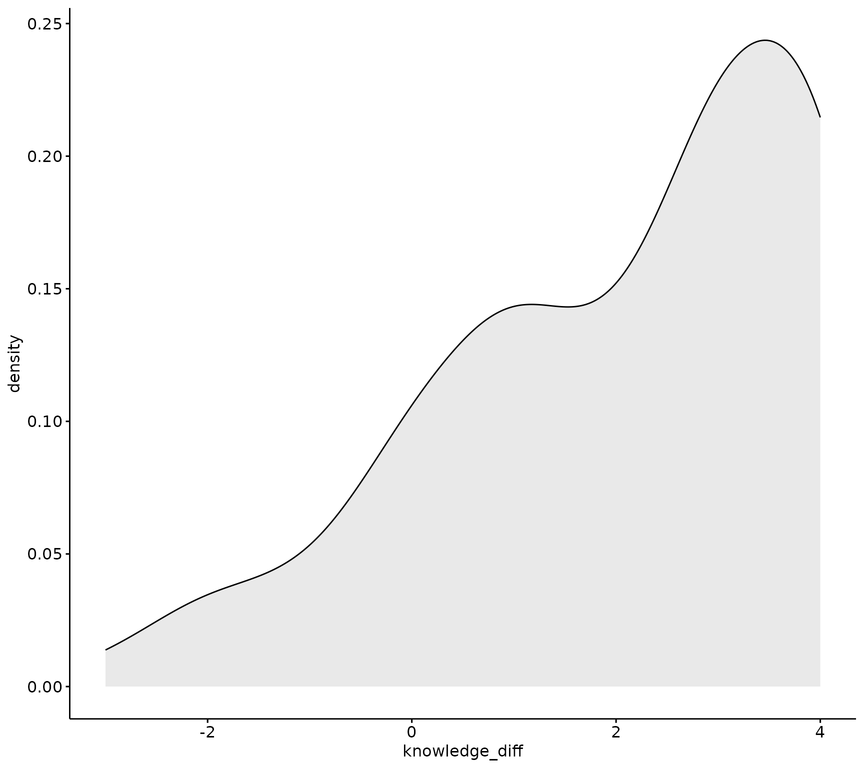
# QQ plot:
ggpubr::ggqqplot(sm_data, "knowledge_diff")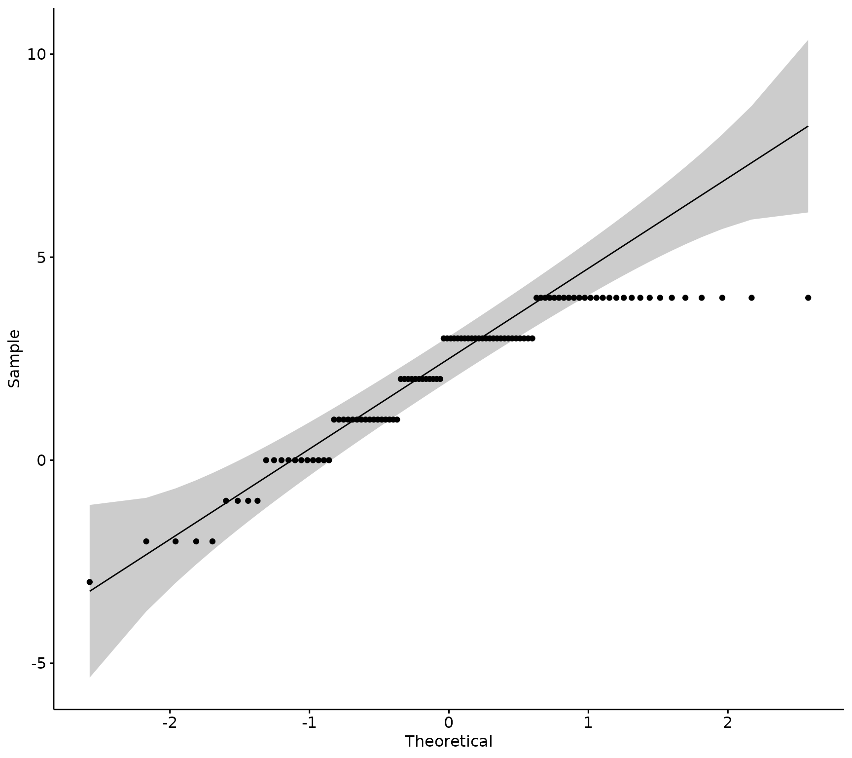
If the data is normally distributed, the density plot would be shaped like a bell curve and the QQ plot would have all of the sample observations (points), lined up along the 45-degree reference line within the shaded confidence interval.
This data is probably not distributed normally, lets run a statistical test to confirm.
Next, run the Shapiro-Wilk’s test. The null hypothesis of this test is the sample distribution is normal. That means that if the test is significant (p-value < 0.05), the distribution is non-normal.
sm_data %>% rstatix::shapiro_test(knowledge_diff)
#> # A tibble: 1 × 3
#>   variable       statistic           p
#>   <chr>              <dbl>       <dbl>
#> 1 knowledge_diff     0.885 0.000000301
rstatix::shapiro_test() returns a tibble with three
column, the column named p is the p-value for the Shapiro’s
test.
Data is not normally distributed for the knowledge items (since the p-value is < 0.05)- use a Wilcoxon test.
Wilcoxon test
There are a couple of ways to run a Wilcoxon test- either a
pipe-friendly version rstatix::wilcox_test() or base R has
wilcox.test where you must pass each variable as a numeric vector.
# Either use a pipe-friendly version of `wilcox_test()` from `rstatix`, need to covert to long form and have `timing` as a variable:
knowledge_wilcoxon <- sm_data %>% dplyr::select(tidyselect::contains("_knowledge") & tidyselect::contains("_num")) %>%  # select the data
                                  tidyr::pivot_longer(tidyselect::contains(c("pre_", "post_")), names_to = "question", values_to = "response") %>% # pivot to long-form
                                  tidyr::separate(.data$question, into = c("timing", "question"), sep = "_", extra = "merge") %>% # Separate out the prefix to get timing
                                  rstatix::wilcox_test(response ~ timing, paired = TRUE, detailed = TRUE) # Run the Wilcoxon test using column "response" (numeric values) on "timing" (pre or post)
knowledge_wilcoxon
#> # A tibble: 1 × 12
#>   estimate .y.   group1 group2    n1    n2 statistic        p conf.low conf.high
#> *    <dbl> <chr> <chr>  <chr>  <int> <int>     <dbl>    <dbl>    <dbl>     <dbl>
#> 1     2.50 resp… post   pre      100   100     3800. 1.23e-13     2.00      3.00
#> # ℹ 2 more variables: method <chr>, alternative <chr>
# Or use the simple base R wilcox.test with each pre and post item:
wilcox.test(sm_data[["post_knowledge_num"]], sm_data[["pre_knowledge_num"]], paired = TRUE)
#>
#>  Wilcoxon signed rank test with continuity correction
#>
#> data:  sm_data[["post_knowledge_num"]] and sm_data[["pre_knowledge_num"]]
#> V = 3800, p-value = 0.0000000000001
#> alternative hypothesis: true location shift is not equal to 0
Wilcoxon test is significant, there is a significant difference in pre and post scores of knowledge scores.
Composite Scales (multiple items)
Most of the surveys we conduct use composite scales of items that measure any underlying concept. These are average together to create a more reliable measure that can then be used in statistical inference.
Creating Composite Scores
Create composite scores for pre and post data by taking the mean of each set of items, and then get difference scores between pre and post mean:
sm_data <- sm_data %>% dplyr::rowwise() %>% # Get the mean for each individual by row
    dplyr::mutate(pre_research_mean = mean(dplyr::c_across(tidyselect::contains("pre_research_") & tidyselect::contains("_num"))), # pre mean for each individual
                  post_research_mean = mean(dplyr::c_across(tidyselect::contains("post_research_") & tidyselect::contains("_num"))), # post mean for each individual
                  diff_research = post_research_mean - pre_research_mean # get difference scores of pre and post means.
    ) %>% dplyr::ungroup()
Normality Testing of Composite Scales
Run a visual inspection of the difference scores between pre and post mean of the research items:
# Density plot:
ggpubr::ggdensity(sm_data, "diff_research", fill = "lightgray")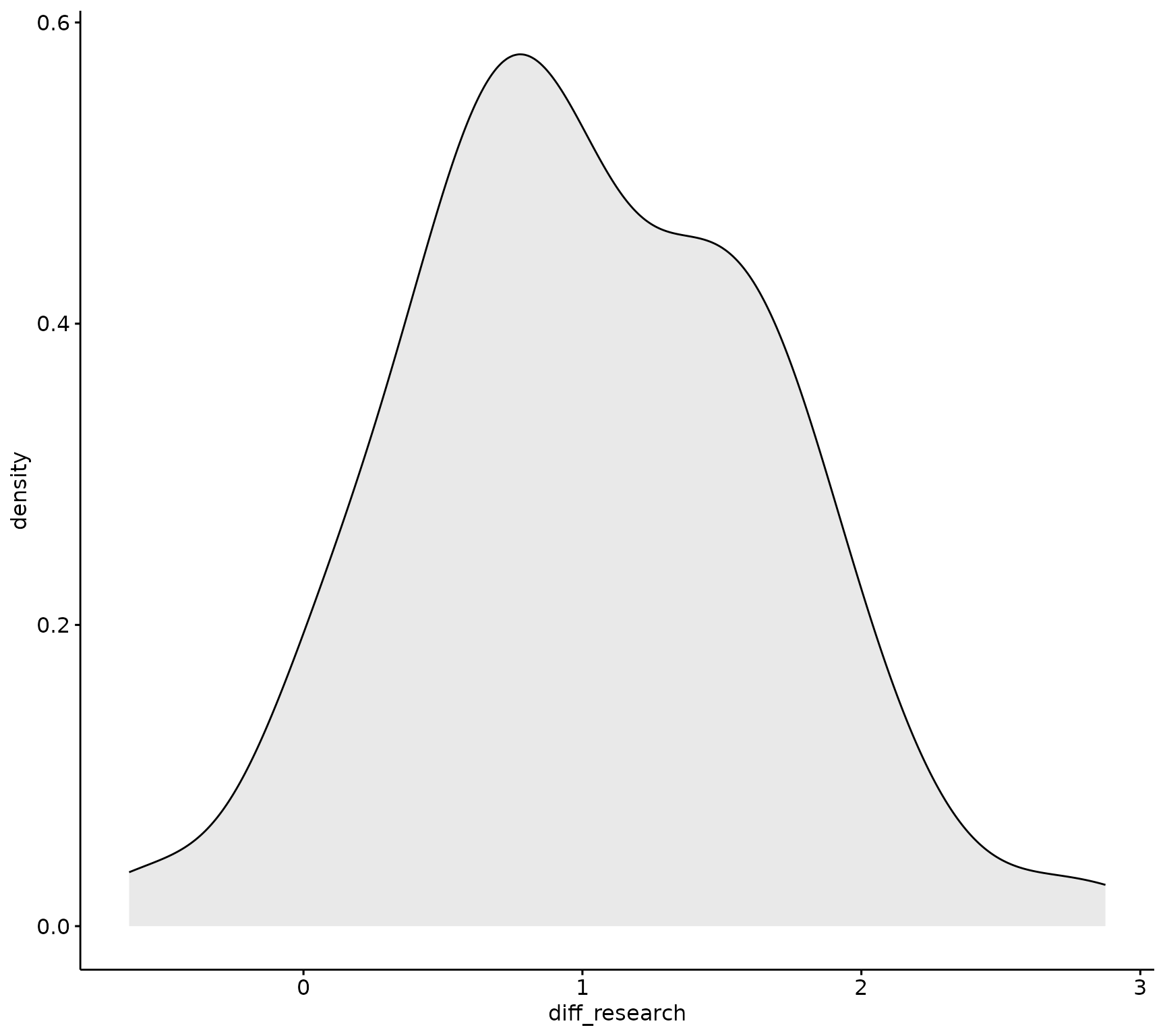
# QQ plot:
ggpubr::ggqqplot(sm_data, "diff_research")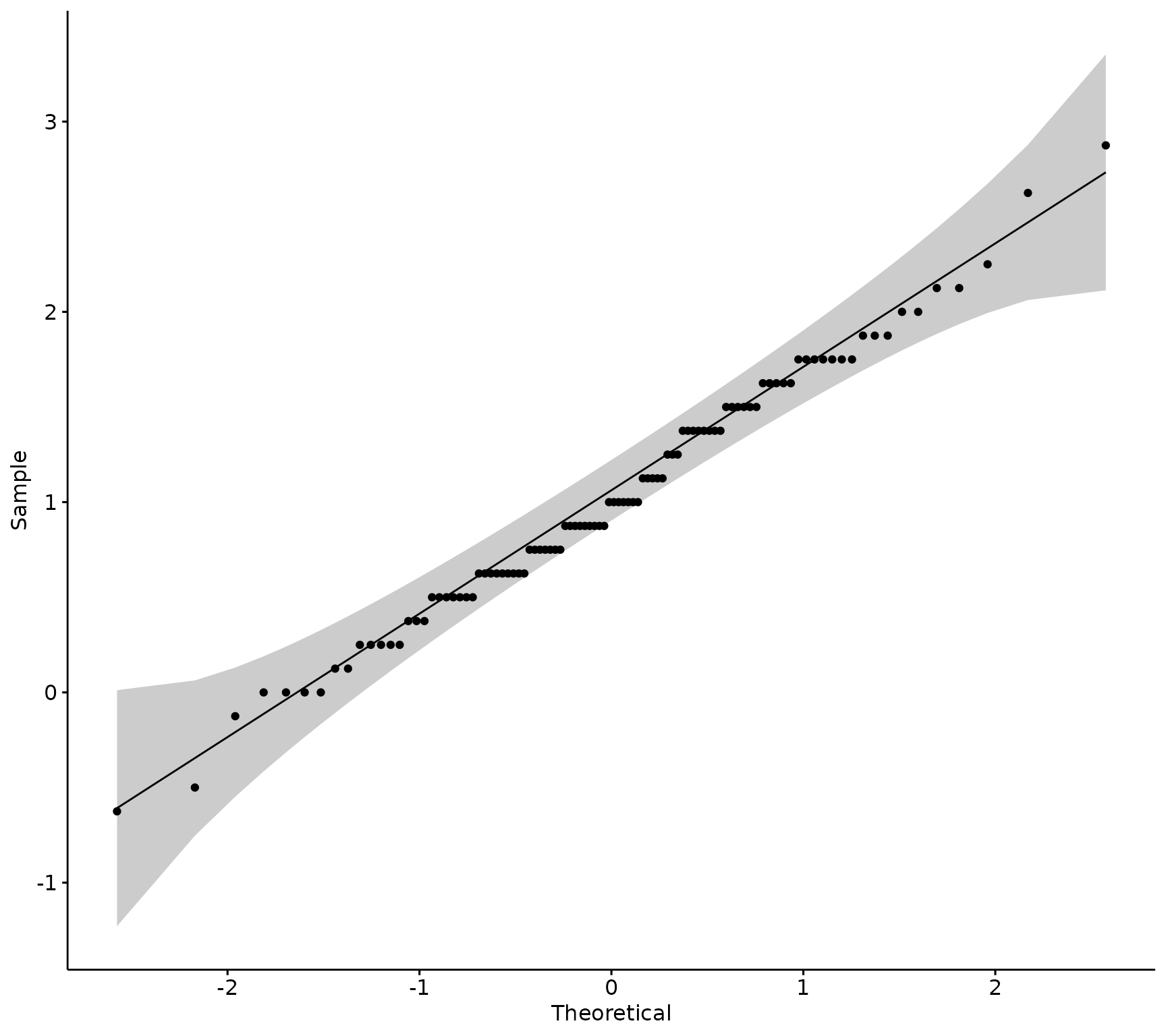
Visually, the data appears normally distributed, Next, run the Shapiro-Wilk’s test to confirm.
sm_data %>% rstatix::shapiro_test(diff_research) # not significant, data likely normal
#> # A tibble: 1 × 3
#>   variable      statistic     p
#>   <chr>             <dbl> <dbl>
#> 1 diff_research     0.991 0.720
Data is normally distributed for the research composite items (since the p-values is > 0.05)- use a T-test.
T-test of Composite Scales
# Either use a pipe-friendly version of wilcox_test from `rstatix`, need to covert to long form and have `timing` as a variable:
research_t_test <- sm_data %>% dplyr::select(pre_research_mean, post_research_mean) %>% # select the pre and post means for research items
                               tidyr::pivot_longer(tidyselect::contains(c("pre_", "post_")), names_to = "question", values_to = "response") %>% # pivot to long-form
                               tidyr::separate(.data[["question"]], into = c("timing", "question"), sep = "_", extra = "merge") %>% # Separate out the prefix to get timing
                               rstatix::t_test(response ~ timing, paired = TRUE, detailed = TRUE)# Run the T-test using column "response" (numeric values) on "timing" (pre or post)
research_t_test
#> # A tibble: 1 × 13
#>   estimate .y.      group1 group2    n1    n2 statistic        p    df conf.low
#> *    <dbl> <chr>    <chr>  <chr>  <int> <int>     <dbl>    <dbl> <dbl>    <dbl>
#> 1     1.02 response post   pre      100   100      15.6 2.43e-28    99    0.890
#> # ℹ 3 more variables: conf.high <dbl>, method <chr>, alternative <chr>
# Or use the simple base R wilcox.test with each pre and post item:
t.test(sm_data[["post_research_mean"]], sm_data[["pre_research_mean"]],  paired = TRUE)
#>
#>  Paired t-test
#>
#> data:  sm_data[["post_research_mean"]] and sm_data[["pre_research_mean"]]
#> t = 16, df = 99, p-value <0.0000000000000002
#> alternative hypothesis: true mean difference is not equal to 0
#> 95 percent confidence interval:
#>  0.8899 1.1501
#> sample estimates:
#> mean difference
#>            1.02
T-test is significant, there is a mean difference in pre and post scores of 1.02.
The vignette Data Visualization will
explain how to create visuals using blackstone with the
example data analyzed in this vignette.