Introduction to blackstone • blackstone

Blackstone Research and Evaluation uses the R programming language as its main tool for data analysis and visualization. The main goal of blackstone is to make the process of coding in R as efficient as possible for everyone at Blackstone Research and Evaluation.

In order to reach this goal, blackstone leverages established R packages and the tidyverse family of R packages in particular. These packages use the system of “tidy data” to make data manipulation and analysis in R consistent and well organized, blackstone also strives to follow this philosophy.

The vignettes provided with blackstone will go into greater detail as to how to use blackstone alongside these other packages. The Setup and R Projects vignette will show you how to set up an R project as well as other standard workflow setups.

This document introduces you to blackstone and how it fits into the basic workflow of data analysis and visualization at Blackstone Research and Evaluation.

Overview of Data Workflow

Import and clean data from survey provider: vignette("import_clean").
Simple data analysis and statistical inference: vignette("analysis").
Data visualization and output for report writing: vignette("data_visualization").

Importing data from SurveyMonkey

Our current survey provider is SurveyMonkey, blackstone contains several functions that makes the process of reading SurveyMonkey data into R a more manageable process and creates a codebook for the data along the way.

SurveyMonkey exports data with two header rows, which does not work with R, where tibbles and dataframes can only have one row of names.

Here is how to import data from SurveyMonkey using example data provided with blackstone, this is a fake dataset of a pre (baseline) survey.

There are three steps to this process:

Create a codebook.

# File path for pre example data:
pre_data_fp <- blackstone::blackstoneExample("sm_data_pre.csv")
# 1. Create the codebook:
codebook_pre <- blackstone::createCodebook(pre_data_fp)
codebook_pre
#> # A tibble: 33 × 5
#>   header_1      header_2 combined_header position variable_name
#>   <chr>         <chr>    <chr>              <int> <chr>        
#> 1 Respondent ID NA       Respondent ID          1 respondent_id
#> 2 Collector ID  NA       Collector ID           2 collector_id 
#> 3 Start Date    NA       Start Date             3 start_date   
#> 4 End Date      NA       End Date               4 end_date     
#> 5 IP Address    NA       IP Address             5 ip_address   
#> # ℹ 28 more rows

For this codebook, the first column header_1 is the first header from the SurveyMonkey data, the second column header_2 is the second header, the third column combined_header is the combination of the two headers, position is the column number position for each combined_header, and variable_name is a cleaned up version for combined_header and will be the column to edit to change the column names later on to shorter and more meaningful names.

variable_name will be the column that renames all the variables in the SurveyMonkey data.

Edit the codebook to create meaningful variable names.

# Step 2. Edit the codebook: 
# Set up sequential naming convections for matrix-style questions with shared likert scale response options:
# 8 items that are matrix-style likert scales- turned into a scale called `research`- here is how to easily name them all at once:
# Rows 11 to 18 belong to the "research" matrix question (you will have to look at the codebook and match the header_1 and header_2 to variable_name to change)
research_items <- codebook_pre[["variable_name"]][11:18]
research_names <- paste0("research_", seq_along(research_items)) %>% purrr::set_names(., research_items) # Create a new named vector of names for these columns
# 6 items that are matrix-style likert scales- turned into a scale called `ability`- Rows 19 to 24 named `variable_name`:
ability_items <- codebook_pre[["variable_name"]][19:24]
ability_names <- paste0("ability_", seq_along(ability_items)) %>% purrr::set_names(., ability_items) # Create a new named vector of names for these columns
# 6 items that are matrix-style likert scales- turned into a scale called `ethics`- Rows 19 to 24 named `variable_name`:
ethics_items <- codebook_pre[["variable_name"]][25:29]
ethics_names <- paste0("ethics_", seq_along(ethics_items)) %>% purrr::set_names(., ethics_items) # Create a new named vector of names for these columns
# Edit the `variable_names` column: Use dplyr::mutate() and dplyr::case_match() to change the column `variable_name`:
codebook_pre <- codebook_pre %>% dplyr::mutate(
    variable_name = dplyr::case_match(
        variable_name, # column to match
        'custom_data_1' ~ "unique_id", # changes 'custom_data_1' to "unique_id"
        'to_what_extent_are_you_knowledgeable_in_conducting_research_in_your_field_of_study' ~ "knowledge",
        'with_which_gender_do_you_most_closely_identify' ~ "gender",
        'what_is_your_current_role_in_the_program' ~ "role",
        'which_race_ethnicity_best_describes_you_please_choose_only_one' ~ "ethnicity",
        'are_you_a_first_generation_college_student' ~ "first_gen",
        names(research_names) ~ research_names[variable_name], # takes the above named vector and when the name matches, applies new value in that position as replacement.
        names(ability_names) ~ ability_names[variable_name],   # Same for `ability_names`
        names(ethics_names) ~ ethics_names[variable_name],   # Same for `ability_names`
        .default = variable_name # returns default value from original `variable_name` if not changed.
        )
    )
codebook_pre
#> # A tibble: 33 × 5
#>   header_1      header_2 combined_header position variable_name
#>   <chr>         <chr>    <chr>              <int> <chr>        
#> 1 Respondent ID NA       Respondent ID          1 respondent_id
#> 2 Collector ID  NA       Collector ID           2 collector_id 
#> 3 Start Date    NA       Start Date             3 start_date   
#> 4 End Date      NA       End Date               4 end_date     
#> 5 IP Address    NA       IP Address             5 ip_address   
#> # ℹ 28 more rows
# Write out the edited codebook to save for future use-
# Be sure to double check questions match new names before writing out:
# readr::write_csv(codebook_pre, file = "{filepath-to-codebok}")

Read in the data and rename the variables with the codebook.

# 3. Read in the data and rename the vars using readRenameData(), passing the file path and the edited codebook:
pre_data <- blackstone::readRenameData(pre_data_fp, codebook = codebook_pre)
pre_data
#> # A tibble: 100 × 33
#>   respondent_id collector_id start_date end_date   ip_address      email_address
#>           <dbl>        <dbl> <date>     <date>     <chr>           <chr>        
#> 1  114628000001    431822954 2024-06-11 2024-06-12 227.224.138.113 coraima59@me…
#> 2  114628000002    431822954 2024-06-08 2024-06-09 110.241.132.50  mstamm@hermi…
#> 3  114628000003    431822954 2024-06-21 2024-06-22 165.58.112.64   precious.fei…
#> 4  114628000004    431822954 2024-06-08 2024-06-09 49.34.121.147   ines52@gmail…
#> 5  114628000005    431822954 2024-06-02 2024-06-03 115.233.66.80   franz44@hotm…
#> # ℹ 95 more rows
#> # ℹ 27 more variables: first_name <chr>, last_name <chr>, unique_id <dbl>,
#> #   knowledge <chr>, research_1 <chr>, research_2 <chr>, research_3 <chr>,
#> #   research_4 <chr>, research_5 <chr>, research_6 <chr>, research_7 <chr>,
#> #   research_8 <chr>, ability_1 <chr>, ability_2 <chr>, ability_3 <chr>,
#> #   ability_4 <chr>, ability_5 <chr>, ability_6 <chr>, ethics_1 <chr>,
#> #   ethics_2 <chr>, ethics_3 <chr>, ethics_4 <chr>, ethics_5 <chr>, …

The SurveyMonkey example data is now imported with names taken from the codebook column variable_name:

names(pre_data)
#>  [1] "respondent_id" "collector_id"  "start_date"    "end_date"     
#>  [5] "ip_address"    "email_address" "first_name"    "last_name"    
#>  [9] "unique_id"     "knowledge"     "research_1"    "research_2"   
#> [13] "research_3"    "research_4"    "research_5"    "research_6"   
#> [17] "research_7"    "research_8"    "ability_1"     "ability_2"    
#> [21] "ability_3"     "ability_4"     "ability_5"     "ability_6"    
#> [25] "ethics_1"      "ethics_2"      "ethics_3"      "ethics_4"     
#> [29] "ethics_5"      "gender"        "role"          "ethnicity"    
#> [33] "first_gen"

The vignette Importing and Cleaning Data goes into deeper detail with example data on how to use blackstone to import and clean data.

Data Analysis and Statistical Inference

First, read in the data that is merged and cleaned in the vignette Importing and Cleaning Data:

# Read in clean SM data:
sm_data <- readr::read_csv(blackstone::blackstoneExample("sm_data_clean.csv"), show_col_types = FALSE)

## Set up character vectors of likert scale levels:
## Knowledge scale
levels_knowledge <- c("Not knowledgeable at all", "A little knowledgeable", "Somewhat knowledgeable", "Very knowledgeable", "Extremely knowledgeable")
## Research Items scale:
levels_confidence <- c("Not at all confident", "Slightly confident", "Somewhat confident", "Very confident", "Extremely confident")
## Ability Items scale: 
levels_min_ext <- c("Minimal", "Slight", "Moderate", "Good", "Extensive")
## Ethics Items scale:
levels_agree5 <- c("Strongly disagree", "Disagree", "Neither agree nor disagree", "Agree", "Strongly agree")

# Demographic levels:
gender_levels <- c("Female","Male","Non-binary", "Do not wish to specify")
role_levels <- c("Undergraduate student", "Graduate student", "Postdoc",  "Faculty")
ethnicity_levels <- c("White (Non-Hispanic/Latino)", "Asian", "Black",  "Hispanic or Latino", "American Indian or Alaskan Native",
                      "Native Hawaiian or other Pacific Islander", "Do not wish to specify")
first_gen_levels <- c("Yes", "No", "I'm not sure")

# Use mutate() for convert each item in each scale to a factor with vectors above, across() will perform a function for items selected using contains() or can be selected 
# by variables names individually using a character vector: _knowledge or use c("pre_knowledg","post_knowledge")
# Also create new numeric variables for all the likert scale items and use the suffix '_num' to denote numeric:
sm_data <- sm_data %>% dplyr::mutate(dplyr::across(tidyselect::contains("_knowledge"), ~ factor(., levels = levels_knowledge)), # match each name pattern to select to each factor level
                                     dplyr::across(tidyselect::contains("_knowledge"), as.numeric, .names = "{.col}_num"), # create new numeric items for all knowledge items
                                     dplyr::across(tidyselect::contains("research_"), ~ factor(., levels = levels_confidence)), 
                                     dplyr::across(tidyselect::contains("research_"), as.numeric, .names = "{.col}_num"), # create new numeric items for all research items
                                     dplyr::across(tidyselect::contains("ability_"), ~ factor(., levels = levels_min_ext)),
                                     dplyr::across(tidyselect::contains("ability_"), as.numeric, .names = "{.col}_num"), # create new numeric items for all ability items
                                     # select ethics items but not the open_ended responses:
                                     dplyr::across(tidyselect::contains("ethics_") & !tidyselect::contains("_oe"), ~ factor(., levels = levels_agree5)),
                                     dplyr::across(tidyselect::contains("ethics_") & !tidyselect::contains("_oe"), as.numeric, .names = "{.col}_num"), # new numeric items for all ethics items
                                     # individually convert all demographics to factor variables:
                                     gender = factor(gender, levels = gender_levels),
                                     role = factor(role, levels = role_levels),
                                     ethnicity = factor(ethnicity, levels = ethnicity_levels),
                                     first_gen = factor(first_gen, levels = first_gen_levels),
                                     )
sm_data
#> # A tibble: 100 × 98
#>   respondent_id collector_id start_date end_date   ip_address      email_address
#>           <dbl>        <dbl> <date>     <date>     <chr>           <chr>        
#> 1  114628000001    431822954 2024-06-11 2024-06-12 227.224.138.113 coraima59@me…
#> 2  114628000002    431822954 2024-06-08 2024-06-09 110.241.132.50  mstamm@hermi…
#> 3  114628000003    431822954 2024-06-21 2024-06-22 165.58.112.64   precious.fei…
#> 4  114628000004    431822954 2024-06-08 2024-06-09 49.34.121.147   ines52@gmail…
#> 5  114628000005    431822954 2024-06-02 2024-06-03 115.233.66.80   franz44@hotm…
#> # ℹ 95 more rows
#> # ℹ 92 more variables: first_name <chr>, last_name <chr>, unique_id <dbl>,
#> #   pre_knowledge <fct>, pre_research_1 <fct>, pre_research_2 <fct>,
#> #   pre_research_3 <fct>, pre_research_4 <fct>, pre_research_5 <fct>,
#> #   pre_research_6 <fct>, pre_research_7 <fct>, pre_research_8 <fct>,
#> #   pre_ability_1 <fct>, pre_ability_2 <fct>, pre_ability_3 <fct>,
#> #   pre_ability_4 <fct>, pre_ability_5 <fct>, pre_ability_6 <fct>, …

Likert Scale Table

The most common task is creating frequency tables of counts and percentages for likert scale items, blackstone has the likertTable() for that:

# Research items pre and post frequency table, with counts and percentages: use levels_confidence character vector
# use likertTable to return frequency table, passing the scale_labels: (can also label the individual questions using the arg question_label)
sm_data %>% dplyr::select(tidyselect::contains("research_") & !tidyselect::contains("_num") & where(is.factor)) %>% 
                blackstone::likertTable(., scale_labels = levels_confidence)

Question	Not at all confident	Slightly confident	Somewhat confident	Very confident	Extremely confident	n
pre_research_1	10 (10%)	8 (8%)	41 (41%)	27 (27%)	14 (14%)	100
pre_research_2	56 (56%)	19 (19%)	8 (8%)	9 (9%)	8 (8%)	100
pre_research_3	32 (32%)	23 (23%)	15 (15%)	20 (20%)	10 (10%)	100
pre_research_4	9 (9%)	24 (24%)	32 (32%)	24 (24%)	11 (11%)	100
pre_research_5	40 (40%)	18 (18%)	21 (21%)	13 (13%)	8 (8%)	100
pre_research_6	17 (17%)	25 (25%)	25 (25%)	16 (16%)	17 (17%)	100
pre_research_7	59 (59%)	13 (13%)	11 (11%)	10 (10%)	7 (7%)	100
pre_research_8	21 (21%)	19 (19%)	23 (23%)	19 (19%)	18 (18%)	100
post_research_1	2 (2%)	26 (26%)	23 (23%)	25 (25%)	24 (24%)	100
post_research_2	12 (12%)	14 (14%)	12 (12%)	14 (14%)	48 (48%)	100
post_research_3	8 (8%)	22 (22%)	21 (21%)	23 (23%)	26 (26%)	100
post_research_4	2 (2%)	24 (24%)	25 (25%)	19 (19%)	30 (30%)	100
post_research_5	14 (14%)	19 (19%)	19 (19%)	19 (19%)	29 (29%)	100
post_research_6	5 (5%)	3 (3%)	24 (24%)	28 (28%)	40 (40%)	100
post_research_7	11 (11%)	10 (10%)	14 (14%)	17 (17%)	48 (48%)	100
post_research_8	4 (4%)	7 (7%)	23 (23%)	23 (23%)	43 (43%)	100

Grouped Demograpic table

blackstone contains a function to create frequency tables for demographics that can be grouped by a variable like role or cohort as well: [groupedTable()].

# Set up labels for variables
# Labels for questions column of table, pass to question_labels argument:
demos_labels <- c('Gender' = "gender",
                  "Role" = "role",
                  'Race/Ethnicity' = "ethnicity",
                  'First-Generation College Student' = "first_gen")

sm_data %>% dplyr::select(gender, role, ethnicity, first_gen) %>% # select the demographic vars
                 blackstone::groupedTable(question_labels = demos_labels) # pass the new labels for the 'Question' column.

Question	Response	n = 1001
Gender
	Female	53 (53%)
	Male	46 (46%)
	Non-binary	1 (1%)
Role
	Undergraduate student	48 (48%)
	Graduate student	23 (23%)
	Postdoc	21 (21%)
	Faculty	8 (8%)
Race/Ethnicity
	White (Non-Hispanic/Latino)	43 (43%)
	Asian	11 (11%)
	Black	18 (18%)
	Hispanic or Latino	12 (12%)
	American Indian or Alaskan Native	7 (7%)
	Native Hawaiian or other Pacific Islander	7 (7%)
	Do not wish to specify	2 (2%)
First-Generation College Student
	Yes	51 (51%)
	No	47 (47%)
	I'm not sure	2 (2%)
1n (%)

Grouped by the variable role:

# Create a group demos table, split by role:
sm_data %>% dplyr::select(gender, role, ethnicity, first_gen) %>% # select the demographic vars
                 blackstone::groupedTable(col_group = "role", question_labels = demos_labels) # pass the new labels for the 'Question' column.

Question	Response	Undergraduate student (n = 48)	Graduate student (n = 23)	Postdoc (n = 21)	Faculty (n = 8)	Total (n = 100)1
Gender
	Female	24 (50%)	13 (57%)	11 (52%)	5 (62%)	53 (53%)
	Male	23 (48%)	10 (43%)	10 (48%)	3 (38%)	46 (46%)
	Non-binary	1 (2%)	-	-	-	1 (1%)
Race/Ethnicity
	White (Non-Hispanic/Latino)	17 (35%)	11 (48%)	10 (48%)	5 (62%)	43 (43%)
	Asian	6 (12%)	2 (9%)	3 (14%)	-	11 (11%)
	Black	11 (23%)	3 (13%)	3 (14%)	1 (12%)	18 (18%)
	Hispanic or Latino	5 (10%)	4 (17%)	2 (10%)	1 (12%)	12 (12%)
	American Indian or Alaskan Native	4 (8%)	-	3 (14%)	-	7 (7%)
	Native Hawaiian or other Pacific Islander	4 (8%)	2 (9%)	-	1 (12%)	7 (7%)
	Do not wish to specify	1 (2%)	1 (4%)	-	-	2 (2%)
First-Generation College Student
	Yes	24 (50%)	11 (48%)	10 (48%)	6 (75%)	51 (51%)
	No	23 (48%)	12 (52%)	10 (48%)	2 (25%)	47 (47%)
	I'm not sure	1 (2%)	-	1 (5%)	-	2 (2%)
1n (%)

Statistical Inference: T-test or Wilcoxon test

Running Normality Test on Single Pre-Post Items

# Use a pipe-friendly version of `shapiro_test()` from `rstatix`, need to covert create a differnce score of post_knowledge_num - pre_knowledge_num named `knowledge_diff`:
sm_data %>% dplyr::select(tidyselect::contains("_knowledge") & tidyselect::contains("_num")) %>%  # select knowledge pre and post numeric items
    dplyr::mutate(knowledge_diff = post_knowledge_num - pre_knowledge_num) %>% # get difference of pre and post scores
    rstatix::shapiro_test(knowledge_diff)
#> # A tibble: 1 × 3
#>   variable       statistic           p
#>   <chr>              <dbl>       <dbl>
#> 1 knowledge_diff     0.885 0.000000301

Data is not normally distributed for the knowledge items (since the p-value is < 0.05)- use a Wilcoxon test.

# Use a pipe-friendly version of `wilcox_test()` from `rstatix`, need to covert to long form and have `timing` as a variable,
# the column named `p` is the p-value:
sm_data %>% dplyr::select(tidyselect::contains("_knowledge") & tidyselect::contains("_num")) %>% 
            tidyr::pivot_longer(tidyselect::contains(c("pre_", "post_")), names_to = "question", values_to = "response") %>%
            tidyr::separate(.data$question, into = c("timing", "question"), sep = "_", extra = "merge") %>% 
            rstatix::wilcox_test(response ~ timing, paired = TRUE, detailed = TRUE)
#> # A tibble: 1 × 12
#>   estimate .y.   group1 group2    n1    n2 statistic        p conf.low conf.high
#> *    <dbl> <chr> <chr>  <chr>  <int> <int>     <dbl>    <dbl>    <dbl>     <dbl>
#> 1     2.50 resp… post   pre      100   100     3800. 1.23e-13     2.00      3.00
#> # ℹ 2 more variables: method <chr>, alternative <chr>

Wilcoxon test is significant, there is a significant difference in pre and post scores of knowledge scores.

The vignette Data analysis and Statistical Inference goes into deeper detail on how to use blackstone to perform more analysis and statistical tests on example data.

Data Visualization

blackstone has functions that create 3 types of charts for data visualization: stacked bar charts, diverging stacked bar charts, and arrow charts.

The functions for stacked bar charts and diverging stacked bar charts can use two different color palettes: a blue sequential palette or a blue-red diverging color palette.

The blue sequential palette should be used for all likert scales that have one clear direction like: Not at all confident, Slightly confident, Somewhat confident, Very confident, Extremely confident

The blue-red diverging color palette should be used if the items have a likert scale that is folded or runs from a negative to positive valence like this: Strongly disagree, Disagree, Neither agree nor disagree, Agree, Strongly agree

This introduction will only show how to create a stacked bar chart, see the vignette Data Visualization for a full explanation of all the data visualization functions in blackstone.

Stacked Bar Charts

The most common visual that is used with reporting at Blackstone Research and Evaluation is a stacked bar chart, blackstone has a function to that makes creating these charts fast and easy: stackedBarChart().

stackedBarChart() takes in a tibble of factor/character variables to turn into a stacked bar chart. The other requirement is a character vector of scale labels for the likert scale that makes up the items in the tibble (same as the one use to set them up as factors in the data cleaning section).

Pre-post Stacked Bar Chart with Overall n and Percentages:

By default, stackedBarChart() uses the blue sequential palette to color the bars and sorts the items by the ones with the highest post items with the highest counts/percentages.

# Research Items scale:
levels_confidence <- c("Not at all confident", "Slightly confident", "Somewhat confident", "Very confident", "Extremely confident")

# select variables and pass them to `stackedBarChart()` along with scale_labels.
sm_data %>% dplyr::select(tidyselect::contains("research_") & !tidyselect::contains("_num") & where(is.factor)) %>% # select the factor variables for the research items
    blackstone::stackedBarChart(., scale_labels = levels_confidence, pre_post = TRUE)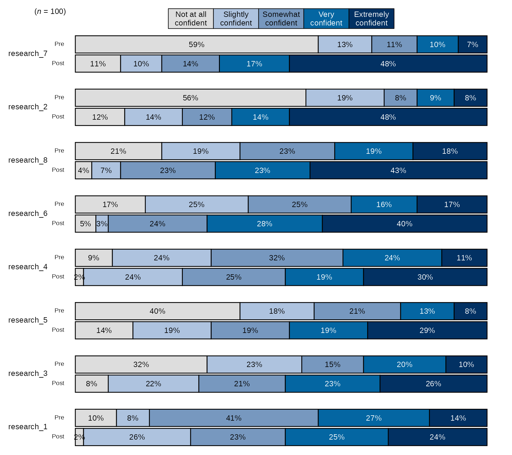

Example of using `blackstone` to create a stacked bar chart with `blackstone::stackedBarChart()`.

The vignette Data Visualization goes into deeper detail on how to use blackstone to create data visualizations with example data.